ETL is THE most important and time-consuming aspect of predictive modelling. An estimated 80% of a data scientist’s time is spent in the ETL stage of model development. Perhaps not as exciting as applying other aspects of the process but the ETL process is critical for quality model development.The old saying is still relevant: "Garbage In Garbage Out"

ETL – Extract, Transform and Load

Real data is messy and needs to be cleansed. The raw data we need for our models will have duplicated data, null fields, inconsistent formats, data input errors and many other general data issues. ‘Clean’ data is a good start but chances are that the data is still not ready for modelling. The data needs to be structured to optimally for the desired data model.

This article highlights a number of standard transformation methods which can be applied when preparing data for a modelling dataset. There is no standard methodology and the data scientist (or ETL developer in this case) needs to know and when to perform the necessary steps.

1. Reduce Size of Data

We should examine the data first. Depending on the dataset size, it may make sense to reduce the size of the initial dataset. We can use PROC SURVEYSELECT to select a random sample of the data.

2. Define a 'Target' variable

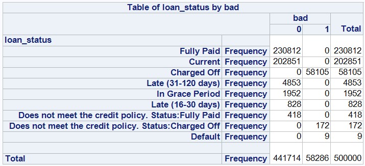
By examining the levels of the chose variable, we can identify the value of interest to our model – in the above example there are three values relating to a bad loan status. We can now transform these values to create a new target variable:

Data transform;

  Set mydata.transactions;

  If loan_status in (‘Charged Off’, ‘Default’, ‘Does not meet the credit policy. Status:Charged Off’) then bad=1; else bad=0;

Run;

One thing to notice here is there are no missing values. In step 3 we discuss imputing missing values however for a target variable this in inadvisable. Take this into account when selecting your target variable.

Using Proc FREQ we can now examine the distribution of the target variable

Proc FREQ Data=transform; TABLES loan_status*bad / nocol norow nopercent; run;

3. IDENTIFYING MISSING NUMERIC DATA

Missing values is one of the most critical issues of data quality. We can use proc MEANS to identify missing values –

PROC Means data=transform N NMISS MIN MAX MEAN;

VAR _NUMERIC_;

OUTPUT OUT=transform_means;

RUN;

4. IDENTIFYING MISSING CHARACTER DATA

Proc FREQ is commonly used to identify missing character data. Some character values will contain many unique values which is not ideal for proc freq, for example ID fields, date fields etc. We can eliminate these values before running proc freq.

PROC FREQ data=transform(drop=ID member_ID start_Date settlement_Date);

TABLES _CHARACTER_;

RUN;

5. Delete variables

After identifying the missing numeric and character variables a decision can be made which variables to keep. A general rule is: variables exceeding 30% of missing values should be dropped. It is inadvisable to try and impute these variables.

6. Value Imputation

We can now try to impute values for the missing values. This is important for several reasons – many algorithms will drop records with missing values on the predictor columns. This will limit the sample size and can lead to the model showing a bias. Since we drop a complete record due to a single missing value we are losing a lot of valuable information.

Numeric Imputation

Mean – replace missing values with the average value.

Median – replace missing values with the mean value.

Mode – replace missing values with the most common value.

Regression – Separate into two groups, missing and non-missing. Use a model on non-missing values to predict values for missing values.

In order to impute missing numeric values with one of the standard statistical values (mean, median, min, max, midrange) the easiest method in SAS is to use PROC STDIZE.

PROC STDIZE DATA=transform REPONLY METHOD=mean OUT=imputed_data; VAR _NUMERIC_;

Character Imputation

The most common method of imputing character variables is to replace any missing values with the most frequent category for that variable. It is helpful to group values using a single character column and produce a cross tabulation using PROC FREQ.

PROC FREQ DATA=transform ORDER=FREQ;

TABLES status*(_CHARACTER_);

RUN;

7. Additional transformations

This article has introduced some basic transformation methods, there are however many more transformations which depending of the quality of the data may be needed for example:

• Transforming character to numeric
• Transforming date values
• Standardization
• Handling outliers
• Creating dummy categories.

Once your data set is properly prepared, the modelling part is likely to be more successful. We will discuss these techniques in a future article. Until then happy ETL-ing!